Siddharth Jain , Cheng Chang ,  Almudena Konrad
( morpheus@eecs.berkeley.edu ,  cchang@eecs.berkeley.edu ,  almudena@cs.berkeley.edu )

Seven Problems

Chapter 8

Solution:
Let H be the Kernel with m rows and n columns, F is the input image with M rows and N columns, and R is the output image with M-m+1 rows and N-n+1 columns. Then we can write R as the convolution of F and H:

where i goes from 1 to M-m+1 and j goes from 1 to N-n+1.
If we assume that H is a square matrix (i.e. n=m) and all the values are ones, then we can write the convolution as:

where C₀=(m-1)/2 for m odd, and C₀=m/2 for m even.
Next, we let 1-C₀=-k and m-C₀=k, so the convolution becomes:

which is Equation 8.1_1, multiplied by  .
The kernel H is a matrix (2k+1) x (2k+1) with all entries being one multiplied by the constant  .

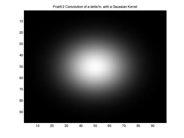
8.2. Write E₀ for an image that consists of all zeros, with a single one at the center. Show that convolving this image with the kernel:

 
 
 

(which is a discretized Gaussian) yields a circularly symmetric fuzzy blob.

Solution:

8.4. Show that convolving a function with a  function simply reproduces the original function. Next show that convolving a function with a shifted  function shifts the function.

Solution:
Let R(x,y) be the result of convolving F(x,y) with H(x,y).

 
 
 
 
 
 
 

If H(x,y) is a delta function meaning H(u,v)=0 everywhere except H(0,0)=1 then,

 
 
 
 
 
 

Convolving with a delta function simply reproduces the original function.

Next consider a shifted delta function H(x,y)=0 everywhere except at H(x_s,y_s)=1. Then,

 
 
 
 
 
 
 
 
 
 

Therefore, convolving with the shifted delta function shifts the function.

8.6. Aliasing takes high spatial frequencies to low spatial frequencies. Explain why following effects occur:

(a) In old cowboy films that show wagons moving, the wheel often seems to be stationary or moving in the wrong direction (i.e. the wagon moves from left to right and the wheel seems to be turning anticlockwise).

(b) White shirts with thin dark pinstripes often generate a shimmering array of colours on television.

Solution:
All these phenomena are examples of aliasing. If we are sampling a signal and it is varying rapidly, then we have to sample fast enough to avoid losing any information.

(a) Let t1 be the time when first snapshot was taken, and t₂ the time when the second snapshot was taken. If t₂ -t₁ is equal to T which is the time taken by the wheel to make a rotation, then the wheel will appear stationary.
If t2-t1 is slightly less than T then the wheel would appear to rotate in the opposite direction.

(b) Thin dark stripes in a dark background mean a rapidly varying signal whose resolution is of the order of the rgb resolution of pixels on the screen. Since the resolution of the image we want to depict is finer than the resolution of pixels available to us on the monitor this effect occurs.

Chapter 9

9.1. Each pixel value in 500 x 500 pixel image I is an independent normally distributed random variable with zero mean and standard deviation one. Estimate the number of pixels that where the absolute value of the x derivative, estimated by forward differences (i.e.  ) is greater than 3.

Solution:
Let X be the random variable representing the number of pixels with x derivative greater than 3. If each pixel has a forward difference, then the number of pixels (N_p) in the image I equals the number of x derivatives. We need to calculate expected value of X (e.i., E(X)).

Let D_i,j=I_i,j - I_i+1,j , then D_i,j is standard normal with mean zero and variance 2. Let Y_i,j, be the indicator function, where Y_i,j is 1 if the absolute value of D_i,j is greater than 3, and Y_i,j is 0 otherwise. Then,

 
 
 

To calculate  , we look at the standard normal table. However, D_i,j is not normal so we perform a change of variable. Let M_i,j=(D_i,j -mean)/(st. dev)= (D_i,j-0)/sqrt(2). Then,  is equal to calculating  , but M_i,j is normal distributed. We obtain:

Chapter 10

Solution:
Let P be the texture plane and I the image plane. The circle is in the plane P.

If I is parallel to P, then the projection is a circle. But, if I is not parallel to P, then the two planes intersect at a line l (see Figure 10.1). We assume l is th x-axis of both, I and P, and the angle between y and y' is  .

(Figure 10.1)

The equation of the circle on P is  . In Figure 10.1 y' is projected to  , so when  (i.e.,  ),  . Re-writing the circle equation and replacing the y' value, we obtain  which is the equation of the ellipse.

Since  , the tilt direction (from y to y') corresponds to the minor axis. The aspect radio is  .

10.2. We will study measuring the orientation of a plane in an orthographic view, given the texture consists of points laid down by a homogenous Poisson point process. Recall that one way to generate points according to such a process is to sample the x and y coordinate of the point uniformly and at random. We assume that the points from our process lie within a unit square.

(a) Show that the probability that a point will land in a particular set is proportional to the area of that set.

(b) Assume we partition the area into disjoint sets. Show that the number of points in each set has a multinomial probability distribution.

We will now use these observations to recover the orientation of the plane. We partition the image texture into a collection of disjoints sets.

(c) Show that the area of each set, backprojected onto the textured plane, is a function of the orientation of the plane.

(d) Use this function to suggest a method for obtaining the plane's orientation.

Solution:
(a) Let S be the set such that,

The probability that a point lands in S is,

 
 
 

Since x and y are chosen independently, the prob. can be written as product of two terms. x and y are chosen uniformly, meaning f(x) and g(y) are simply constants (say 1) so that,

 
 

Therefore, the probability that a point will land in a particular set S is proportional to the area of the set A(S).

(b) Let S be partition into disjoint sets: {S₁ , ...,S_p}, then

 
 

where N(S_i) denotes the number of points in S_i.
This probability is proportioanal to,

 

where A_i denotes the area of the sub-set S _i and n=n₁+...+n_p.
This is the multinomial probability distribution. The factor  , arises because of all the different ways (combinations) in which we can divide n points so that n₁ is in S₁, n₂ is in S₂, and so on.

(c) Let P be an arbitrary plane whose orientation we want to find. The image plane I is z = 0. We can form P in the following way: start with the plane z=0. Rotate the plane "-vely" about the x-axis by an amount  . This is equivalent to applying a rotation matrix  . Next, rotate the plane about its "local" y-axis by an amount  . This is equivalent to applying  . Thus, the overall transformation is,  , since  .

 
 
 
 
 

Thus the unit normal (0,0,1) is transformed into,

 
 
 

which means that the equation for this plane is  .
If we take any point (x_projected,y_projected ) on the image plane and use orthographic backprojection, then the backprojected point is x = x_projected and y = y_projected, and using the equation of the plane we obtain:

 
 

Note that in our analysis the object plane passes through the origin, but this doesn't lead to any loss of generality.
We are now ready to find out how an area transforms when we backproject it from the image plane to the object plane. Consider a rectangle in the  image plane :

 
 
 

The backprojection of vertices is:

 
 
 
 
 

To find backprojected area we do the following analysis:

 
 
 
 
 
 
 

Therefore, the backprojected area is a function of the orientation of the plane.

(d) In an orthographic projection, A_i increases by the same multiplicative factor by which A_j increases (A _i is the area of the set S_i). To find the orientation of the plane we experimentaly divide the image plane into random disjoint sets S_i having area A_i. We count the number of points n _i which land in each set. Then if we use orthographic (back)projection then the probability that we obtain the observation we got is proportional to:

 

which is proportional to  . Unfortunately this doesn't help in determining and  .

If we used some other projection (eg. perspective instead of orthographic), then when we backproject, different areas on the image plane get scaled by different amounts. We form:
,

where n₁, ... , n_p are known by observation. We choose that  and  such that they maximize the probability of the observation we got. These values will give the orientation of the plane (which was our objective). 

Three Programming Assignments
10.3. Texture synthesis: Implement the non-parametric texture synthesis algorithm of section 10.3.2. Use your implementation to study:

(a) the effect of window size on the synthesized texture;
(b) the effect of window shape on the synthesized texture;
(c) the effect of the matching criterion on the synthesized texture (i.e., using weighted sum of squares instead of sum of squares, etc.).

Solution:
First consider the i/p file description:
The i/p file "file.dat" is of the form:

w1.xmin w1.xmax w1.ymin w1.ymax
w2.xmin w2.xmax w2.ymin w2.ymax sigma
EPSILON CONST3
rows cols
data file
o/p filename

Example of an i/p file (e.g., bread6.dat)
-1 1 -1 1
-6 6 -6 6 2.0
0.1 0.2
225 225
bread.gray
bread6.out

The first line specifies the size of the initial seed used to synthesize the image. In the above example we are saying,  start by putting a 3X3 seed from the template

The second line specifies the size of the window used for comparing pixels - this parameter has to be chosen cleverly and varies from image to image. We incorporate a Gaussian weighting in the code so that errors due to nearby pixels in the window(w2) are emphasized more than the errors due to distant pixels. For this the user has to i/p sigma of the Gaussian - this also has to be chosen cleverly.

The third line represents two other parameters choosing which is again guesswork and which are pretty critical. The first, EPSILON is a number such that all points satisfying d <= (1+EPSILON)*dmin are saved and then the bestmatch is randomly chosen from the pool of saved points.

Consider two points p1, p2 which give the same rms (root mean square) distance. Further suppose for p1 the no. of terms (rms distance = sqrt( sum_{1,N} square_of_diff / N )) N in the computation was 10 whereas p2 also gave same distance but N was just 1. Clearly we don't want to save p2. Therefore we have to incorporate some form of weighting to avoid p2 getting saved (e.g., d = (rms distance)/sqrt(N) - this is roughly what we do).

Consider another case in which p1 and p2 both give d equal to zero and again N was 10 for p1 and 1 for p2. The simple multiplicative weighting above will not work in this case - what we can do is to replace zero by a small number - this is the value of CONST3.

The fourth line specifies the size of image to synthesize (rows*cols).

The fifth line specifies i/p filename to the program which has rgb values of the pixels.

The sixth line specifies o/p filename of the file to be generated by the program.

The algorithm is notoriously slow as it grows the image pixel by pixel. The maximum time required to generate an o/p file of 225*225 pixels was more than 40 hrs. Because of the time constraint we were not able to experiment extensively with the parameters EPSILON, CONST3, and w2.

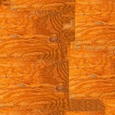
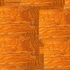
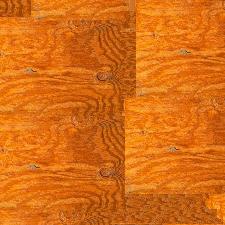
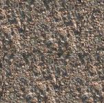
(a) The effect of varying the window size is illustrated in following figures:
"wood4.jpg" , generated using a window of 9*9 pixels. See i/p parameters: "wood4.dat"
"wood5.jpg" , generated using a window of 11*11 pixels. See i/p parameters: "wood5.dat"
"wood6.jpg" , generated using a window of 13*13 pixels. See i/p parameters: "wood6.dat"
The template file (file used to synthesize the image) is "wood.gif" .

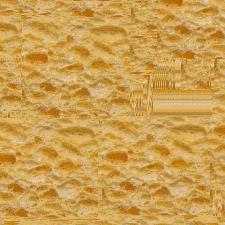
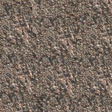
Another set of examples:
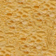
"bread4.jpg" , generated using a window of 9*9 pixels. See i/p parameters: "bread4.dat"
"bread5.jpg" , generated using a window of 11*11 pixels. See i/p parameters: "bread5.dat"
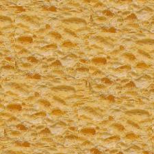
"bread6.jpg" , generated using a window of 13*13 pixels. See i/p parameters: "bread6.dat"
The template file is "bread.gif" .

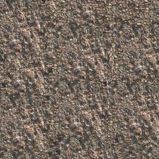
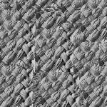
(b) Effect of window shape:
"bumpy2_p3.jpg" , generated using a square window of 11*11 pixels. See i/p parameters: "bumpy2_p3.dat"
"bumpy2rect.jpg" , generated using a rectangular window of 13*9 pixels. See i/p parameters: "bumpy2rect.dat"
The template file is "bumpy2.gif" .

(c) The effect of matching criterion:
"bumpy2_p3.jpg" , generated incorporating a Gaussian weighting (with sigma = winsize/6.4) to emphasize errors due to nearby pixels more than the errors due to far away pixels. See i/p parameters:"bumpy2_p3.dat" .
"bumpy2_p1.jpg" , generated without incorporating any Gaussian weighting. See i/p parameters: "bumpy2_p1.dat" .

More examples:
"D181.jpg" (see i/p parameters: "D181.dat" ).

"D18.gif"

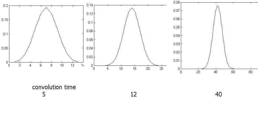
8.7. One way to obtain a Gaussian kernel is to convolve a constant kernel with itself, many times. Compare this strategy with evaluating a Gaussian kernel.
(a) How many repeated convolutions will you need to get a reasonable approximation? (you will need to establish what a reasonable approximation is; you might plot the quality of the approximation against the number of repeated convolutions).
(b) Are there any benefits that can be obtained like this?

Solution:
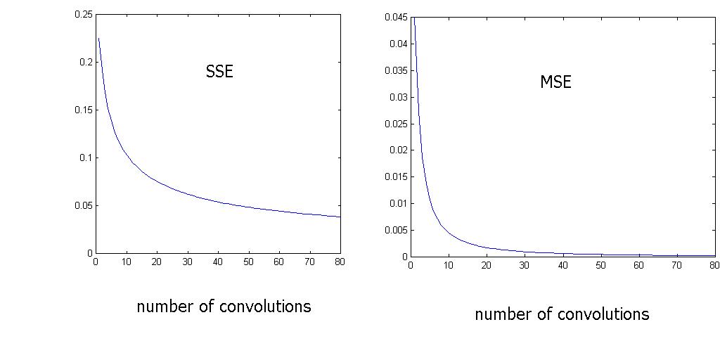
(a) Figure "convolution.jpg" , shows the convolution of the constan kernel with itself 5, 12 and 40 times.
Figure "diagram.jpg" , shows the sum of square-error(SSE) from the approximation to the evaluation of the Gaussian function, where SSE= Sum ((approximation(i)- evaluation(i)) ^2).
The evaluation gaussian function has the same mean and variance with the approximation kernel MSE=SE/(length of the kernel).

(b) The convolution method does not need the computer to compute exponential of a float number, it only requires the computer to do multiplication and summation.
All the original kernel have length 3.

8.8. Write a program that produces a Gaussian pyramid from an image.

Solution:
The Matlab files for the code are:
"gauss_f.m"
"gaussianpyramid.m"
"upsample.m"

We run the code on two images:
Zebra image.
Arch image.