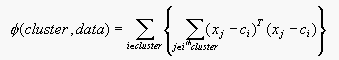
(Equation 15.1)
used in Section 15.4.2 may be inappropiate - for example, colour differences could be too strongly weighted if colour and texture are measured on different scales.
Siddharth JainĀ, Cheng Chang ,ĀAlmudena Konrad
( morpheus@eecs.berkeley.edu,Ā
cchang@eecs.berkeley.edu,Ā almudena@cs.berkeley.edu
)
Five Problems
15.1. We wish to cluster a set of pixels using
colour and texture differences. The objective function
(Equation 15.1)
used in Section 15.4.2 may be inappropiate - for example, colour
differences could be too strongly weighted if colour and texture are
measured on different scales.
(a) Extend the description of the k-means algorithm to deal with
the case of an objective function of the form
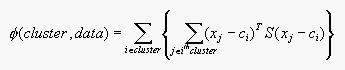
(Equation 15.2)
where S is an a symmetric, positive definite matrix.
(b) For the simpler objective function, we had to ensure that each cluster contained at least one element (otherwise we can't compute the cluster center). How many elements must a cluster contain for the more complicated objective function?
(c) As we remarked in section 15.4.2, there is no guarantee that k-means gets to a global minimun of the objective function; show that it must always get to a local minimum.
(d) Sketch two possible local minima for a k-means clustering method clustering data points described by a two-dimensional feature vector. Use an example with only two clusters, for simplicity. You shouldn't need many data points. You should do this exercise for both objective function.
Solution:
(a) In these equations xj is the feature vector
representing the jth data point and ci is the
centroid. By adding the matrix S, we can put a weight to the color and
texture features. Let
xj-ci=zji. Then
Equation 15.2 can be written as:
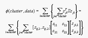
where zij,1 represents the color difference between jth
data point and the centroid, and zij,2 represents the
texture difference between jth data point and the centroid. And
s12 = s21. By chosing
the values in S we can put weight in the color and texture features.
In the k-means algorithm, the data points are assigned at random
to the K sets. Then the centroid is computed for each set. These two
steps are alternated until there is no further change in the
assignment of the data points. This process converge to a local
minimun of the objective function (Equation 15.2).
(b) For both objective functions we need at least one data point in each cluster.
(c) Assume a dataset where each point has two features. Figure 1
illustrates an example.Let the number of clusters k be 3, and the
number of points is 7. Then, we can choose at random one of the
following cluster centers
{123,124,125,126,127,128,134,135,136,137,145,146,147,156,157,167}. By
calculating Equation 15.1 with all the possible cluster center, we
find the a local minimum to be clusters {1,7,5} with cluster 1 having
three points{1,4,6}, cluster 7 has two points {7,3} and cluster 5 has
point {5,2}.
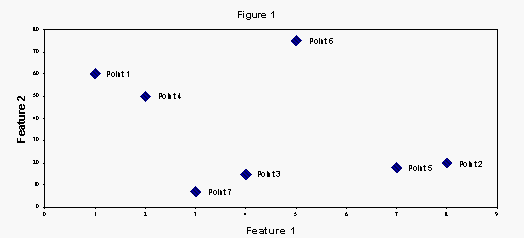
(d) For the example in part (c) two local minimum are: clusters
{(1,4,6),(7,3),(5,2)}, and clusters {(1,4),(7,3),(6,5,2)}.
For the case of Equation 15.2, the local minimum will depend on
the values we choose for the matrix S, which will put weights on each
feature. But the procedure to find the local minimum will be the same.
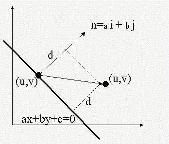
16.1. Prove the simple, but extremely useful, result that the perpendicular distance from a point (u,v) to a line (a,b,c) is given by abs(au+bv+c) if a^2+b^2=1.
Solution:
Let P=(x1,y1) be apoint in the line
ax+by+c=0. The normal vector to this point in the line is
n=ai+bj, this vector is perpendicular to the line
(see Figure 2). The distance d is equal to the length of the
orthogonal projection of the vector p from point P to point (u,v) on the
normal vector n. The equation for d is:
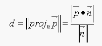
where,
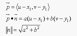
so the equation for d becomes:
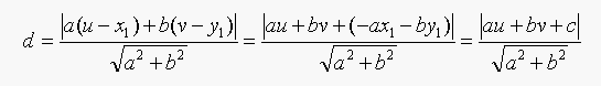
So if a^2+b^2=1, then d=|au+bv+c|;
ĀĀFigure 2.
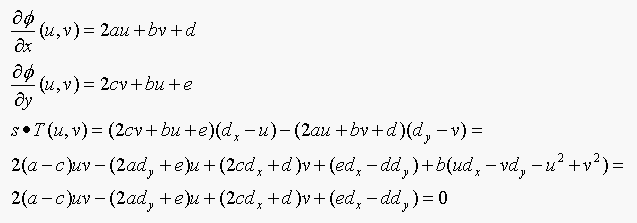
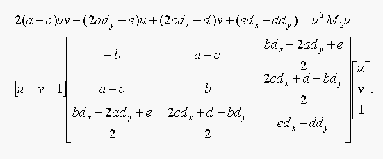
16.5. A conic section is given by 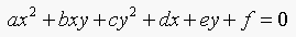 .
.
(a) Given a data point (dx,dy), show that the
nearest point on the conic (u,v) satisfies two equations:
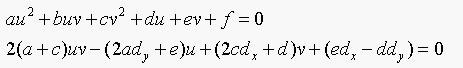
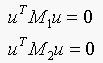
(b) These are two quadratic equations. Write u for the
vector (u,v,1). Now show that for M1 and M2, we
can write these equations as:
Solution:
(a) The point (u,v) in on the conic section, therfore substituing
u and v for x and y in the conic section equation we satisfied the
first equation. To satisfy the second equation we follow the analysis
in pag 454 in the book. The normal at a point (u,v) is:

evaluated at (u,v). We must satisfiy T.s=0, where T
is the tangent to the curve, and
s=(dx,dy)-(u,v) is normal to the curve.
(b)
The first equation in matrix form:
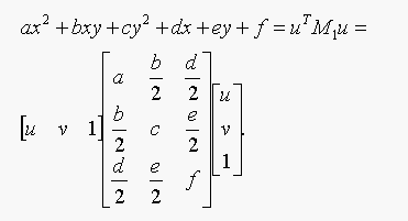
The second equation in matrix form:
16.6. Show that the curve
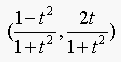
is a circular arc (the length of the arc depending on the interval for
which the parameter is defined).
(a) Write out the equation in t for the closest point on this arc to some data point (dx,dy); what is the degree of this equation? How many solutions in t could there be?
(b) Now substitute  in the
parametric equation, and write out the equation for the closest point
on this arc to the same data point. What is the degree of the
equation? why is it so high? What conclusions can you draw?
in the
parametric equation, and write out the equation for the closest point
on this arc to the same data point. What is the degree of the
equation? why is it so high? What conclusions can you draw?
Solution:
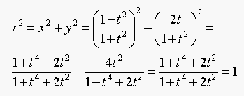
The parametric equation for the circle is:

If we let r=1,  , and
, and  , then the parametric equation becomes:
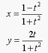
To verify we show that  :
:
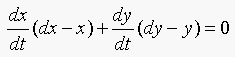
(a) The vector from the closest point on the curve to the data
point is normal to the curve. Following the analysis in page 457 in
the book the equation in t for the closest point to the arc is:
 (Equation 16.6)
where,
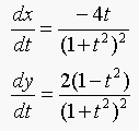
Equation 16.6 becomes:
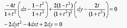
The degree of the equation is 2.
(b) Solving Equation 16.6 with gives:
which has degree 8.
18.3. We said that
(Equation 18.3)
Show that this is true. The easiest way to do this is to take logs
and rearrange the fractions.
Solution:
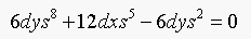
The left hand side os Equation 18.3 is:
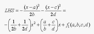
The right hand side of Equation 18.3 is:
And the LHS = RHS if and only if
Three Programming Assignments
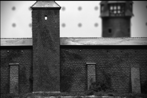
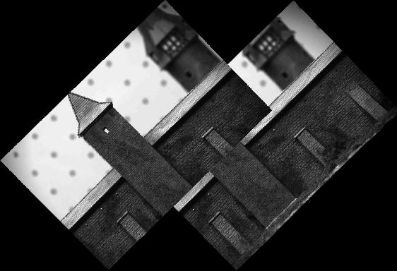
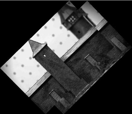
12.11. Implement the rectification process.
We rectified 2 images of those. We choose "http://www-2.cs.cmu.edu/afs/cs.cmu.edu/project/cil/ftp/cil-0003/images/c-000302.gif",
and "http://www-2.cs.cmu.edu/afs/cs.cmu.edu/project/cil/ftp/cil-0003/images/c-000311.gif".
The calibration data are "http://www-2.cs.cmu.edu/afs/cs.cmu.edu/project/cil/ftp/cil-0003/calib/c-000302.par", and "http://www-2.cs.cmu.edu/afs/cs.cmu.edu/project/cil/ftp/cil-0003/calib/c-000311.par".
The new image plane is parellel to the plane spanned by the baseline (the line connecting two camera centers) and the intersecting line of the 2 old image planes. The equation of the new image plane is : [ 0.00700976172873 0.12882591610886 0.99164244895992]*[x,y,z]'= R. And the new x-axis in the new image plane is parallel to the baseline.
The new rotation matrix from world coordinate to camera coordinate:
[ 0.71020742428920 0.69746714719922 -0.09562945708453 ]
[ -0.70395758233363 0.70494216920007 -0.08660404354588 ]
[ 0.00700976172873 0.12882591610886 0.99164244895992 ]
The rectificatoin result: (The old image plane has R as -1977)
1) R= -1885 "result1.jpg". The new image
plane is at the same side as old image planes from the camera centers.
2) R= -189 "result2.jpg". The new image
plane is at the same side as old image planes from the camera centers.
3) R= -2640 "result3.jpg". The new image
plane is at the opposite side as old image planes from the camera
centers.
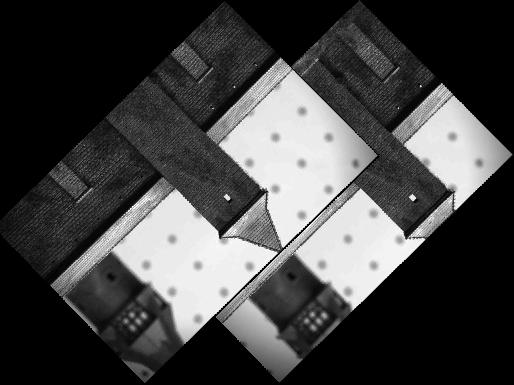
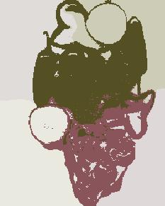
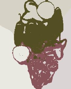
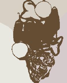
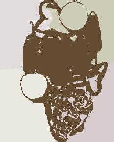
15.7. Implement a segmenter that uses k-means to form segments based on colour and position. Describe the effect of different choices of the number of segments; investigate the effects of different local minima.
Solution:
implementing the K-means segmentation algorithm
In our algorithm, we do not select K manually. Instead, we add a penalty function to the objective funtion, square_root_of (K * number_of_feature)/32. Here , number_of_feature=5 (2 position and 3 color features). And in the objective funtion, we normalized all the features.
Next we minimize the objective function over both clustering and K.
Experiment results:
In Figure "original1.jpg", there are 2
different segmentations (3 different local minimums). All with K=6
(optimal K). The results are shown in Figures "seg1_6_1.jpg" and "seg1_6_2.jpg".
Next, we fix K=3,4,5. The results are illustrated in the following
figures:
"seg1_3.jpg", "seg1_4.jpg", and "seg1_5.jpg".
We provide two more examples:
"original2.jpg" => "seg2.jpg", and
"original3.jpg" => "seg3.jpg".
16.9. Implement a hough transform line finder.
Solution:
The program is consists of 2 parts
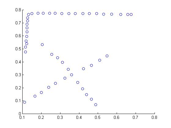
Part A) Extract points from an image (see Figure "original_points.jpg").
Part B) Extract line structures using Hough Transform.
B.1) Vote process other than the range of angle and R in the book.
We used the range of R from[- sqrt(2),sqrt(2)], the range of angle from [0,
PI). The steps are 1/200 of the ranges in both angle and R.
Notice: in this setup, two line structures are very similar when
they lie at leftmost and rightmost of the vote plane, meanwhile their
y-coordinates are opposite. You will see it in the
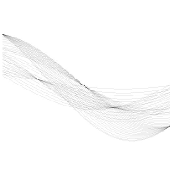
example. See Figure "vote_result.jpg".
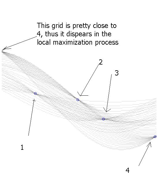
B.2) Local maximization, find the grid which has the most votes in
a local 5*5 window, meanwhile the grid has more than 6(threshold set
manually) votes.
Note: sometimes there are more than 1 grid have
the property above, then merge them. See Figure "local_maximization.jpg".
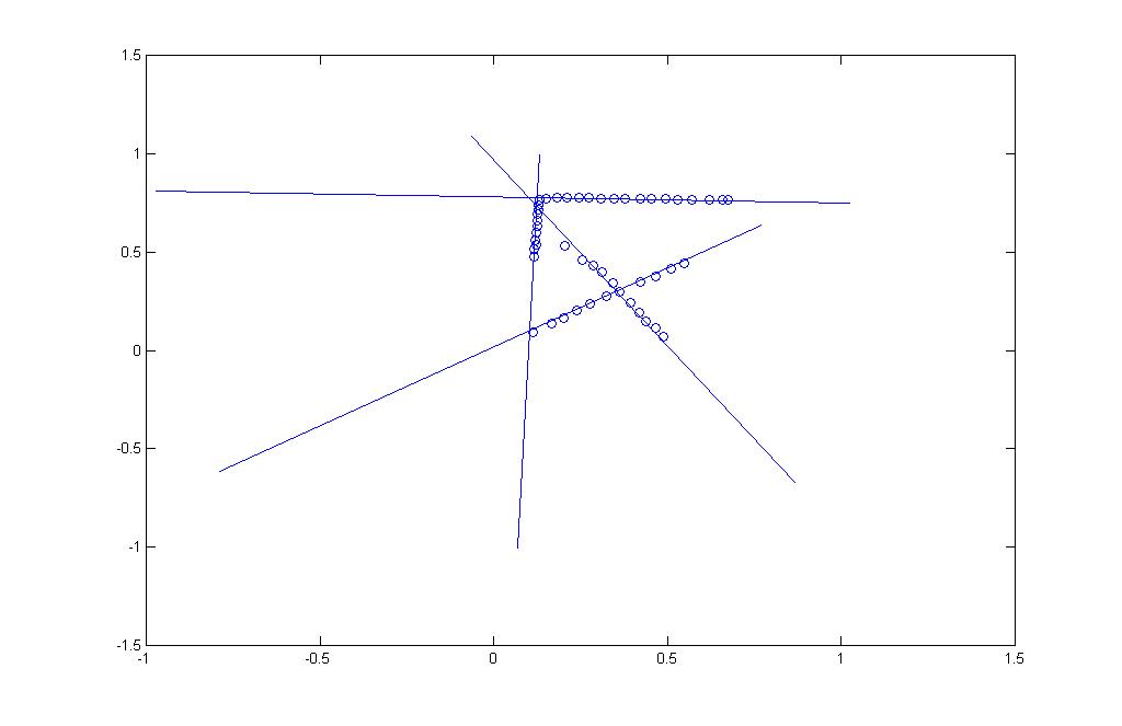
B.3) According to the angle and R of the line, extract the line. See Figure "line_structure.jpg".