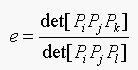
(Equation 20.2)
is an affine invariant (as long as no two of i, j, k and l are the same, and no three of these points are collinear).
Siddharth JainĀ, Cheng Chang ,ĀAlmudena Konrad
( morpheus@eecs.berkeley.edu,Ā
cchang@eecs.berkeley.edu,Ā almudena@cs.berkeley.edu
)
Seven Problems
20.2. We have a set of plane points Pj; these are
subject to a plane affine transformation. Show that:
(Equation 20.2)
is an affine invariant (as long as no two of i, j, k and l are the
same, and no three of these points are collinear).
Solution:
Pi is of the form 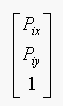 (in homogeneous coordinates).
Let C denote the plane affine transformation, then
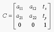
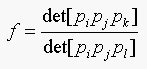
If e is an affine invariant then f should be equal to e. Where f is:
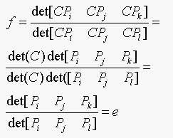
Therefore e is an affine invariant. The assumptions
that no two of i, j, k and l are the same and no three points are
collinear, are required so that det[Pi Pj
Pk] and det[Pi Pj Pl] are nonzero.
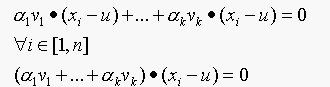
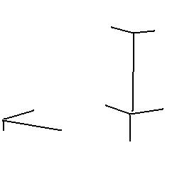
20.4. In chamfer matching, at any step, a pixel can be updated if the distance from some or all of its neighbours to an edge are known; Borgefors counts the distance from a pixel to a vertical or horizontal neighbour as 3 and to a diagonal neighbour as 4 to ensure the pixel values are integers. Why does this mean sqrt(2) is approximated as 4/3? Would a better approximation be a good idea?
Solution:
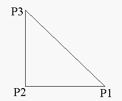
In the figure above P2 is a neighboring horizontal
pixel, and P3 is a neighboring diagonal pixel.
In terms of exact math and using Pythagoras' Theorem:
Borgefors approximates P1P2 as 3 and
P1P3 as 4, for integer arithmetic. So
 is approximated as 4/3, (i.e,
sqrt(2) is approximated as 4/3).
is approximated as 4/3, (i.e,
sqrt(2) is approximated as 4/3).
A better approximation is P1P2 as 10 or 5
(instead of 3), and P1P3 as 14 or 7 (instead of 4).
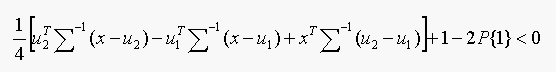
24.1. Assume that we are delaing with measurements x in some feature space S. There is an open set D where any element is classified as class one, and any element in the interior of S-D is classified as class two.
(a) Show that
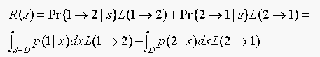
(b) Why are we ignoring the boundary of D (which is the same as the boundary of S-D) in computing the total risk?
Solutions:
(a) The probability that given x it is of class 1 but lies in S-D
is = P{1->2 | using s}
The probability that given x it is of class 2 but lies in D is = P{2->1 | using s}
Therefore,

(b)The boundary is a break-even point. The type I and type II errors both give the same risk, so we don't have any preference over comitting type I or type II error. This means that if a point lies on the boundary, we can classify it as belonging to either class 1 or class 2. We have no preference, so we ignore the boundary of D in computing the total risk.
24.2. In section 2, we said that, if each class-conditioanl density had the same covariance, the classifier of algorithm 2 boiled down to comparing two expressions that are linear in x.
(a) Show that this is true.
(b)Show that, if there are only two classes, we need only test the
sign of a linear expression in x.
Solution:
(a) Our strategy is to choose the class k with the smallest value of
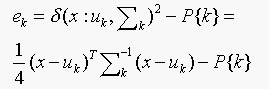
If  is the same for all the
classes then,
is the same for all the
classes then,
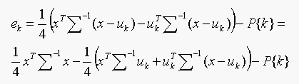
We have to choose the class which gives minimum ek. Since
 is common to all
ek, its effect cancels out and our strategy simplifies to
choosing the class which gives the minimum value of
is common to all
ek, its effect cancels out and our strategy simplifies to
choosing the class which gives the minimum value of 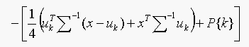 ,
,
which is linear in x.
(b) Only two classes,
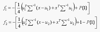
Test: Choose class 1 if f1 < f2,
else choose class 2.
Test:Classify as belonging to class 1 if
Thus, we need only to test the sign of a linear expression in x.
24.3. In section 24.3.1, we set up a feature u, where the value
of u on the ith data point is given by 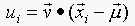 . Show that u has zero mean.
Solution:
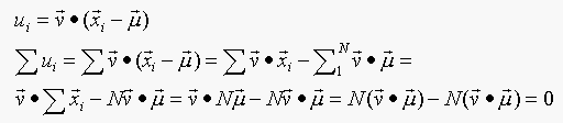
Therefore, u has zero mean.
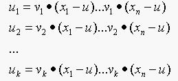
24.4. In section 24.3.1, we set up a series of feature u, where
the value of u on the i'th data points is given by . We then said that the v would be eigenvectors of  , the covariance matrix of the data items. Show taht
the different features are independent, using the fact that the
eigenvectors of a symmetric matrix are orthogonal.
, the covariance matrix of the data items. Show taht
the different features are independent, using the fact that the
eigenvectors of a symmetric matrix are orthogonal.
Solution:
Consider 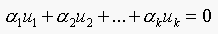 .
.
This means,
Since
dotting above with vj and using the fact that
eigenvectors of a symmetric matrix are orthogonal, we have  , since
  , if
, if  . This implies that
  as
as  . Since
  , then the trivial solution is
  , which implies that
  are independent.
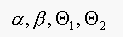
24.5. In section 24.2.1, we said that the ROC was invariant to choice of prior. Prove this.
Solution:
To prove that ROC is invariant to prior, we first consider the case
when 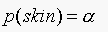 . Our decision rule is:
If 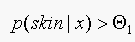 , classify as "skin",
using Baye's rule this is equivalent to
, classify as "skin",
using Baye's rule this is equivalent to 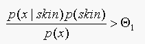 .
.
So if 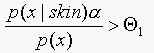 classify as "skin",
otherwise classify as "not skin".
classify as "skin",
otherwise classify as "not skin".
Consider a second case when 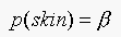 . The decision rule becomes:
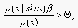 classify as "skin",
otherwise classify as "not skin".
classify as "skin",
otherwise classify as "not skin".
 should be
  , to get the same performance. Note that
 are all positive, thus the
ROC is invariant to choice of prior.
are all positive, thus the
ROC is invariant to choice of prior.
BTW 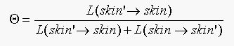 .
.
where skin'=not skin.
Two Programming Assignments
Chapter 22. Build Finder Programming Assignment.
Solution:
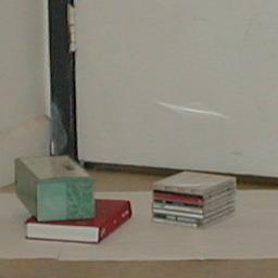
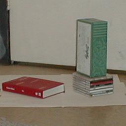
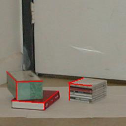
If we have an orthographic camera, the image of a cuboid (length, width, depth may be different) object has nice properties. Assume the 3 edges of the cuboid which intersect at the same corner are x,y,z axis respectively. Then we can recover the rotation matrix R from the image of those 3 edges on the image plane. After abtaining the rotation matrix R, we can further recover the length of the 3 edges.
This is simple geometry, the idea are showed in the codes: "compute_length.m" and "compute_rotation.m".
Experiments:
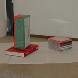
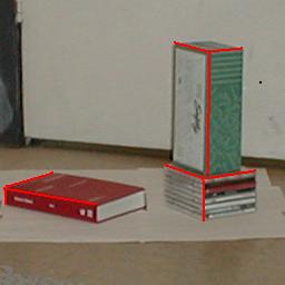
Observation1: The objects are far away, and they all have the same
distance from the PIN_HOLE camera. Their images on the image plane can
be roughly treated as orthographic images. Based on this obervation,
we took several pictures of a bunch of cuboid objects from a FAR away
but the same distance. Next, we labeled the 3 edges by hand (in fact,
the corner could be any of the 8 corners). Then, we recover the length
of the edges.
Result: The orginal images are
raw1.jpg, raw2.jpg, and
raw3.jpg.
The distance of the objects from the camera is greater than 20
times of the objects depth. So it can be thought as an orthographic camera.
We manually labeled with edges, label1.jpg,
label2.jpg, and label3.jpg.
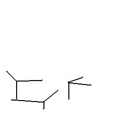
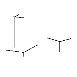
And extract the edges to edge1.jpg,
edge2.jpg, and edge3.jpg.
For each cuboid, we compute the rotation_matrix, then we recover the actual length(in pixel) of the 3 edges of that cuboid.
Results:
Image 1:
13.4208, 70.2794, 101.024
61.0692, 56.1338, 38.5388
57.0870, 36.7850, 112.0122
Image 2:
13.5964, 103.9230, 66.5207
102.6300, 54.0617, 32.4556
34.5076, 59.1464, 51.8748
Image 3:
34.7967, 50.7668, 58.3267
36.7273, 51.9904, 108.1041
14.4606, 100.1409, 68.9547
So, we can tell which objects are corresponding in different images. And clearly we can say:
1st in image1 == 1st in image2 == 3rd in image3
2nd in image1 == 3rd in image2 == 1st in image3
3rd in image1 == 2nd in image2 == 2nd in image3
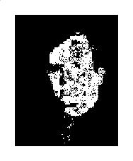
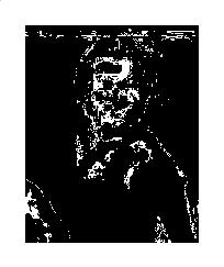
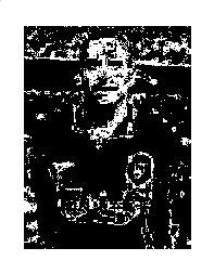
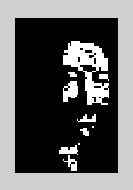
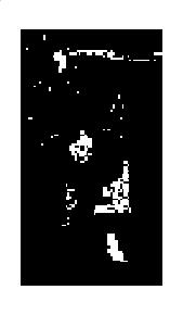
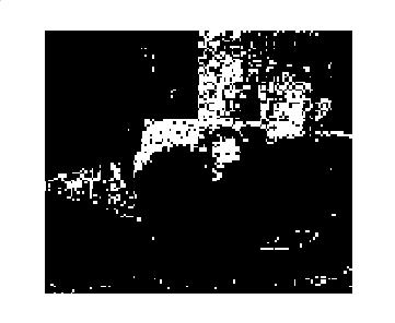
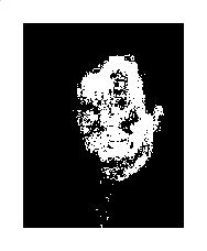
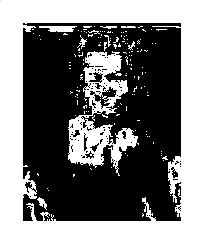
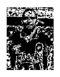
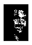
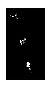
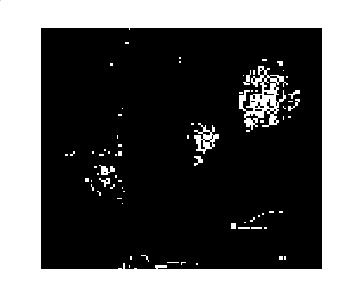
Chapter 26. Skin detector Programming Assignment.
Solution:
We implemented 2 skin detectors. The skin data is from 40 pictures
collected from the Internet. And the non-skin data is from around 3,000 pictures from Corel data.
Method1: Nearest Neighbor.
We cluster all those skin-pixels into 150 clusters, and the non_skin-pixels
into 500 clusters. Notice that each cluster has different weight, according
on how many pixels in the training-pictures are clustered into that cluster.
Next, we process a new image (independent of the training set).
For each pixel of the image, we find the nearest neighbor of that
pixel from all those 650 centers. And, if the neartest one is skin,
then we report skin, otherwise we report non_skin.
The advantage of this method is that is fast, and the disadvange
is that it dosn't work well in some instances, especially when the color of that pixel is on the boundary of skin-non_skin area.
Method2: K-nearest Neighbor
We cluster all those skin-pixels into 150 clusters, and the non_skin-pixels
into 500 clusters. Notice that each cluster has different weights, according
on how many pixels in the training-pictures are clustered into that cluster.
Next, we process a new image (independent of the training set).For
each pixel of the image, find the nearest K-neighbor of that pixel
from all those 650 Centers. In those K neighbors, we compute the sum of
all those weight of those skin clusters = W_SKIN , then compute the
sum of all those weights of those non_skin clusters =W_non_skin. If
W_skin > W_non_skin, we report skin, otherwise we report non_skin.
The advantage of this method is that it yields better
performance, it is stable, and so far the best skin detector we
found. The disadvange is that is slower compared to the first one.
Experiments: The original pictures are 1.jpg, 2.jpg, 3.jpg, 4.jpg, 5.jpg, and 6.jpg.
The results of method 1 are skin1.jpg, skin2.jpg, skin3.jpg, skin4.jpg, skin5.jpg, and skin6.jpg.
The results of method 2 are
skin1.jpg, skin2.jpg,
skin3.jpg, skin4.jpg,
skin5.jpg, and skin6.jpg.