Siddharth Jain
morpheus@eecs.berkeley.edu

Polygonal Segmentation and Refinement of Aerial Digital Surface Maps

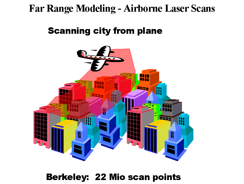
At the Video and Image Processing Laboratory (VIP Lab) we are engaged in automated 3D Model Generation for Urban Environments. A Digital Surface Map (DSM) is constructed by projecting laser scan points, taken from an airplane, to the ground (xy plane) and coding the depth of the scan point by a gray value. Figure 1 shows the schematic of an airplane flying over a city and figure 2 shows the DSM of the north UC Berkeley campus

Figure 1: Aerial Scanning of a city

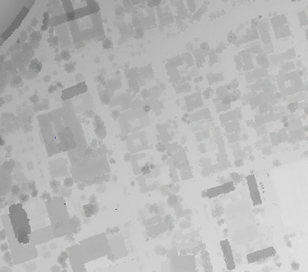
Figure 2: Digital Surface Map of noth UC Berkeley campus

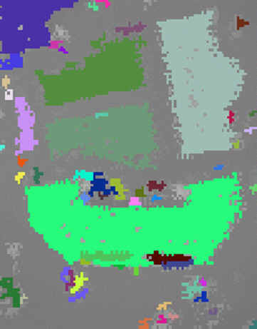
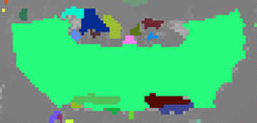
The DSM can be depth segmented using a flood-filling algorithm to give figure 3. In this figure the ground is coded as gray color and every other color corresponds to some depth value.

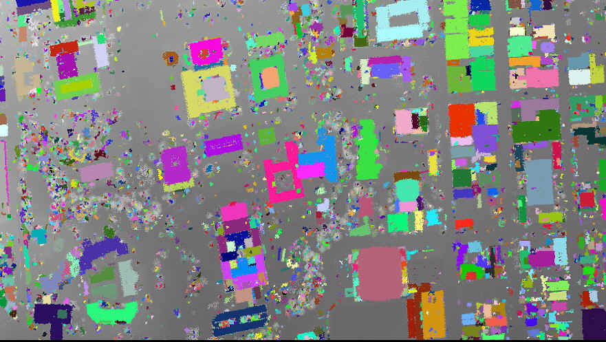
Figure 3: Depth Segmented DSM

The aerial data is very noisy and low resolution. A 3D model using the raw DSM is shown in figure 4

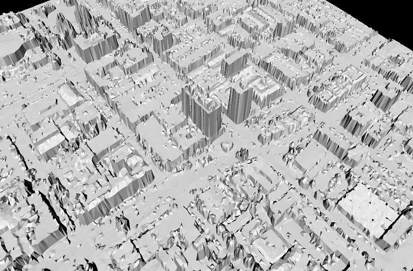
Figure 4: 3D model using raw DSM

Note that the building facades are jagged instead of being straight - this is because of the jaggedness in the building contours of the DSM. The jaggedness in the building facades adversely affecting their texture mapping. Also the roof tops are not planar and pointed cone like structures are prevalent in figure 4 and these correspond to the noisy data points (outliers) in the DSM. Our goal in this project is to fit polygons to the building contours in the DSM, to straighten the contours and to refine the DSM so that the resulting 3D model is more realistic and visually pleasing.

A flowchart giving an overview of the data processing steps is shown below:

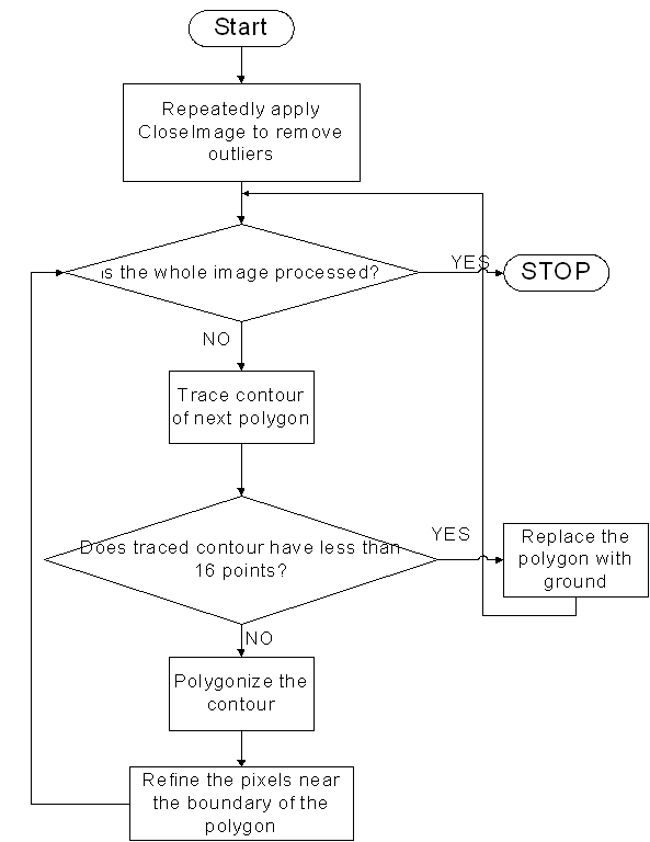
Figure 5: Overview of the data processing steps

We start by applying an operation CloseImage to the image in which for each pixel (x,y) in the image we take a 3x3 window centered at this pixel and construct a histogram of color values. We exclude the center pixel (x,y) in constructing the histogram. If the most commonly occurring color has votes > 4 we replace the color of the center pixel (x,y) with the most commonly occurring color. This is illustrated in figure 6.

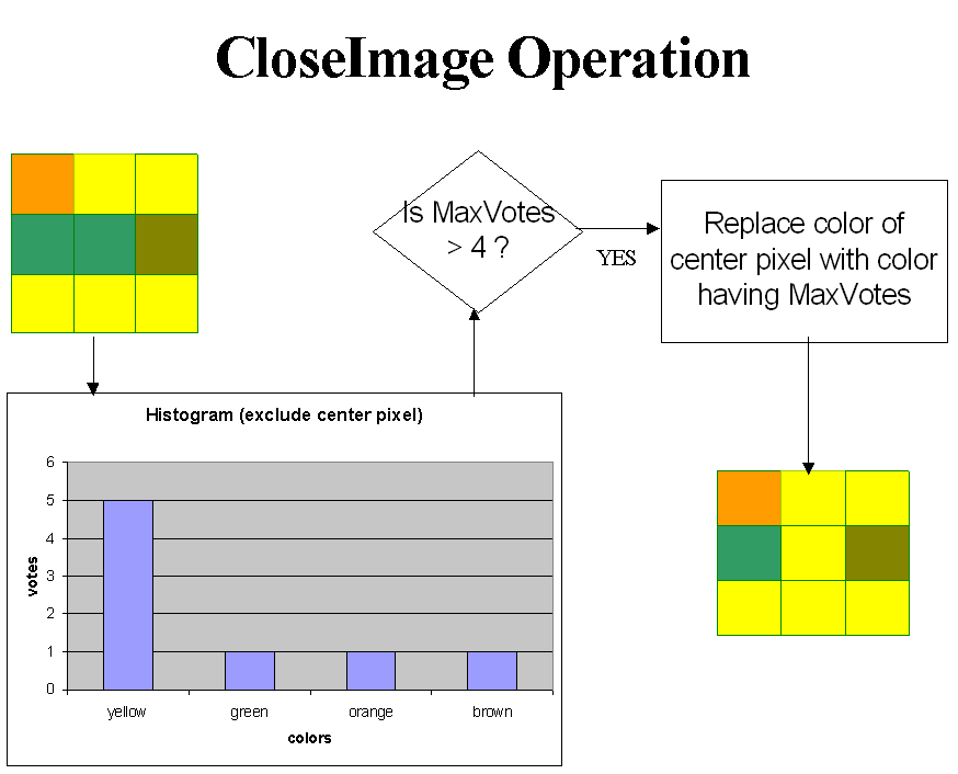
Figure 6: The CloseImage Operation

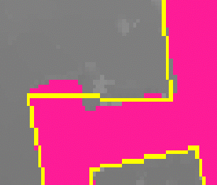
Figure 7 shows close up of a region in the raw DSM and the result after 3 iterations of CloseImage

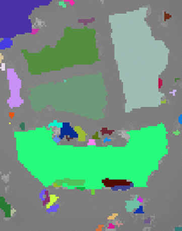
Figure 7: DSM after 3 iterations of CloseImage

After applying 3 iterations of CloseImage we start tracing contours of buildings and fitting polygons to them. A pixel (x,y) is defined as a  boundary point if (1) it is not gray and (2) in the 3x3 window centered at the pixel there is at least one pixel that has color not equal to color of (x,y). We need an auxiliary array A that tells whether a pixel is a boundary pixel or not. A(x,y) = 0 means we don't know whether (x,y) is a boundary pixel or not. A(x,y) = -1 means (x,y) is not a boundary pixel. A(x,y) = 1 means (x,y) is a boundary pixel. We initialize A to 0 and keep updating it as the status of pixels becomes known. Contour Tracing is done using the Radial Sweep algorithm. A good tutorial can be found at http://www.cs.mcgill.ca/~aghnei. As we trace the contour we change A(x,y) of the contour pixels from 0 to 1. The algorithm terminates upon encountering 3 consecutive boundary pixels that have already been marked before i.e. for which A(x,y) is 1. There are a few cases when the algorithm fails. This is illustrated in figure 8.

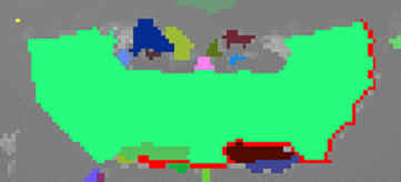
Figure 8: A case when Radial Sweep fails

In such cases we use another algorithm called MarkBdry. Figure 9 shows the order in which Radial Sweep would check points for boundary pixels. The current point is labeled Current and the previous boundary point in the sequence is labeled prev. Instead of using the ordering in Figure 9 MarkBdry uses the ordering shown in Figure 10. 

Figure 9: ordering in Radial Sweep                                        Figure 10: ordering in MarkBdry

Thus MarkBdry tries to keep going in the same direction. Also we try to avoid points that have already been marked before - thus if A(x,y) = 1 for point 1 but A(x,y) = 0 for point 2 and point 2 is a boundary point we insert 2 in the contour sequence instead of 1. The stopping criterion for MarkBdry is same as that for Radial Sweep. Figure 11 shows the contour traced by MarkBdry.

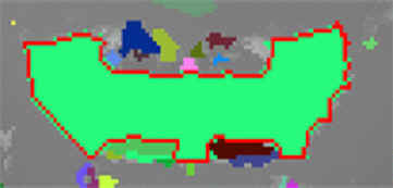
Figure 11: Contour traced by MarkBdry

It is important to note that MarkBdry also fails in some cases - thus we combine Radial Sweep and MarkBdry

After the contour of a polygon is traced and we find that it has less than 16 pixels (corresponding to a small area) we remove the polygon from the image and replace it with ground. Figure 12 shows the flowchart for doing this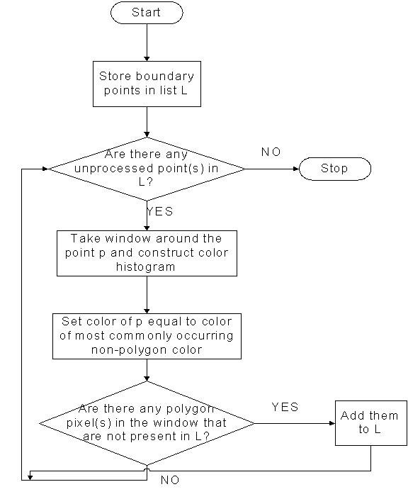                       

Figure 12: Removing small polygons from the DSM

If the contour has more than 40 pixels we fit a polygon to it using the Douglas-Peucker-Ramer algorithm. A good interactive demo can be found at http://cgm.cs.mcgill.ca/~godfried/teaching/projects97/guirlyn/iterEndpoints/frames.html. This is followed by scan converting lines and refining pixel values near the polygonal boundary. First we have to determine the interior and exterior of the polygon. Figure 13 explains how this is done - we count the number of polygon pixels to the left and right of the polygon boundary - the side having higher count is the interior of the polygon.

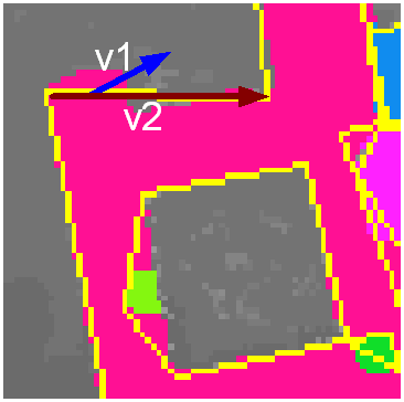
Figure 13: Finding interior and exterior of polygon

Once we have found the interior and exterior we change the color of all non polygon pixels in the interior to the color of polygon and remove polygon pixels lying in the exterior of the segmented polygon. Figure 14 shows the result.

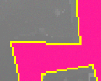
Figure 14: Refining pixel values near the boundary of the polygon

Figure 15 shows the segmented and refined DSM using above data processing techniques.

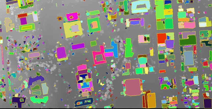
Figure 15: Segmented and Refined DSM

Figure 16 shows 3D Model using the segmented and refined DSM

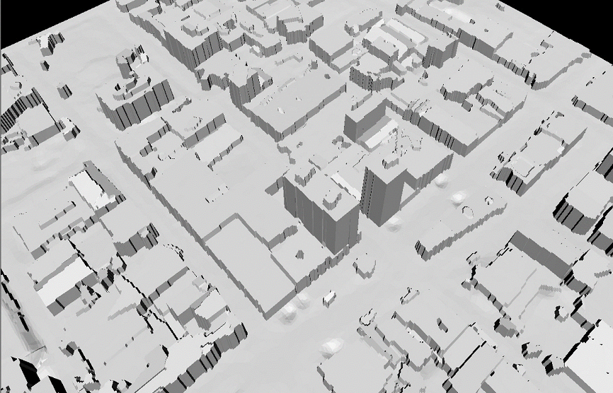
Figure 16: 3D Model using Refined DSM

Acknowledgements: Christian Fruh